While working on atMETEO, I found it useful to bring the measured
temperature and atmospheric pressure values into relation with the position
of the sun or the current moon phase and see how they correlate.
Back then when Grafana only supported the Graphite
datasource this was done with a simple script that calculated those
values every minute and stored them in the Graphite database along with the
other measurements.
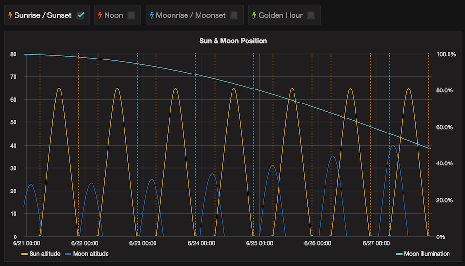
Now that Grafana supports a sophisticated plugin framework (starting
with v3.0), I have created the Sun and Moon Datasource Plugin for
Grafana which uses SunCalc to calculate the position
of sun and moon on demand when rendering on the frontend. Additional features
are the calculation of the moon illumination and annotations for various events
such as sunrise or sunset.
The main advantage of doing the calculation in a datasource on the client side
is that the values don’t have to be pregenerated which is not optimal with
Graphite because it does not allow to submit future values and therefore the
calculation has to be done just in time.
From a technical point of view the plugin is interesting because as of today
it is the only Grafana plugin that doesn’t rely on a server providing the data.
Therefore it might be a useful example for new plugin authors.
Feedback
When submitting the plugin to Grafana.net I received very
positive feedback from raintank, the company behind Grafana and
Torkel Ödegaard even demoed the datasource in his talk at this year’s
Monitorama which happened to take place two days after I
created the Pull Request on GitHub. Thanks for this! A recording is available
on YouTube.
Outlook and further work
The current version of the plugin implements all features that SunCalc
currently offers. Nevertheless there are already a few ideas for future
improvements.
I could imagine that the plugin might be useful when monitoring
photovoltaic systems (maybe even solar parks). For this the calculation
of the clear sky radiation could be added. Additionally the annotations could
be extended to be able to show additional astronomic events such as full and
new moon or solstices/equinoxes and perihelion/aphelion.
If you have additional ideas or want to help out for example with the
calculation of the mentioned values, please use the
issue tracker on GitHub.
I’m running a small Linux server (HP ProLiant MicroServer G7 N54L) in my
home network as backup drive for desktops and notebooks. The health of the
server is critical and therefore I wanted to keep track of some system
metrics such as temperatures, voltages and system fan speed in the hope that
they can detect hardware problems in advance.
These metrics are typically offered by hardware monitor chips and can
be accessed in Linux with the lm-sensors utilities (sensors-detect and
sensors). Unfortunately sensors-detect was not able to detect the
respective chip (Nuvotem/Winbond W83795ADG). After a bit of research, it
turned out that the SMBus/I2C driver for the chipset failed to detect the
sensor. Luckily there was already a patch available that fixed
the driver but supported only an older kernel version. The patch was never
merged into the mainline Linux kernel and meanwhile a few things have changed
in that module. Since I think it’s a valuable change, I ported it to the
current kernel version, cleaned it up and re-sent it to the
mailing list where it’s currently being reviewed. (UPDATE: The
patch has been merged and is included in Linux 4.5.)
For the time being, the patched driver can be found in this GitHub
repository including a more detailed description and
installation instructions. This should make it simple for anyone
interested to test it and use it on their systems.
After installation of the updated driver and loading the modules, sensors is
able to show the measurements:
dg-i2c-1-2f
Adapter: SMBus PIIX4 adapter SDA2 at 0b00
Vcore:        +0.88 V  (min =  +0.50 V, max =  +1.40 V)
Vdimm:        +1.51 V  (min =  +1.42 V, max =  +1.57 V)
+3.3V:        +3.30 V  (min =  +2.96 V, max =  +3.63 V)
3VSB:         +3.26 V  (min =  +2.96 V, max =  +3.63 V)
System Fan:   679 RPM  (min =  329 RPM)
CPU Temp:     +34.8°C  (high = +109.0°C, hyst = +109.0°C)
                       (crit = +109.0°C, hyst = +109.0°C)  sensor = thermal diode
NB Temp:      +43.2°C  (high = +105.0°C, hyst = +105.0°C)
                       (crit = +105.0°C, hyst = +105.0°C)  sensor = thermal diode
MB Temp:      +20.8°C  (high = +39.0°C, hyst = +39.0°C)
                       (crit = +44.0°C, hyst = +44.0°C)  sensor = thermistor
The sensor readings can be easily aggregated with collectd’ssensor plugin. Unfortunately the current version of the
plugin has one minor limitation and tracks the sensor readings only by
metric names (e.g “temp1”) but not by the more descriptive labels
(e.g. “CPU Temp”). To address this shortcoming I’ve created a
pull request on GitHub. (UPDATE: The pull request has been
merged and the feature is included in collectd 5.6.0.)
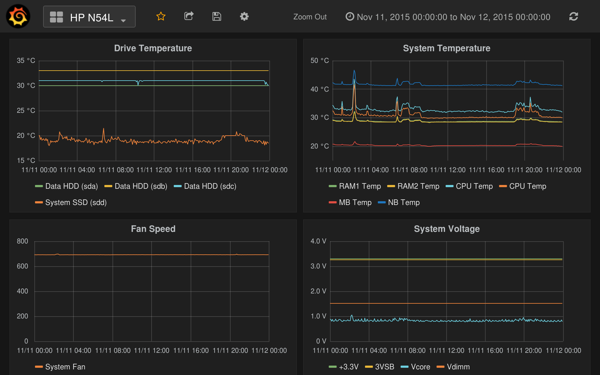
The following grafana screenshot shows the result:
The drive temperatures were collected using the HDDTemp plugin.
Besides logging and visualizing internet connection statistics
I wanted to track also local weather conditions and later eventually integrate
the data into a home automation system. While today there are proprietary and
free projects available that facilitate this, the topic seemed to be a perfect
candidate for a small spare time open source project, which I called
atMETEO.
Project goals and introduction
Programming an ATmega based weather station not only allowed to deepen my
knowledge in electronics and microcontrollers, at the same time the project
served as practical accompaniment while reading Modern C++ Design and
C++ Templates and enabled me to explore the advantages and limits of
modern C++ on 8 bit hardware.
The essential concept of atMETEO is to read and interpret data from
sensors connected to the microcontroller and to transfer this
information to a connected PC for further processing, storing and
visualization.
Ideally atMETEO should hereby be able to access my already existing Hideki
TS53 RF sensors. Therefore a preliminary step was to
reverse engineer their data format.
Conducting test automation is essential in order to develop a stable
product which can be left running unattended. For this purpose a Jenkins
server has been set up that runs Clang Static Analyzer, builds all commits
and executes unit tests (including code coverage generation). In addition it
flashes new software periodically and maintains statistics on successful and
failed attempts to read sensor data for a given time range to identify possible
race conditions.
Technical aspects
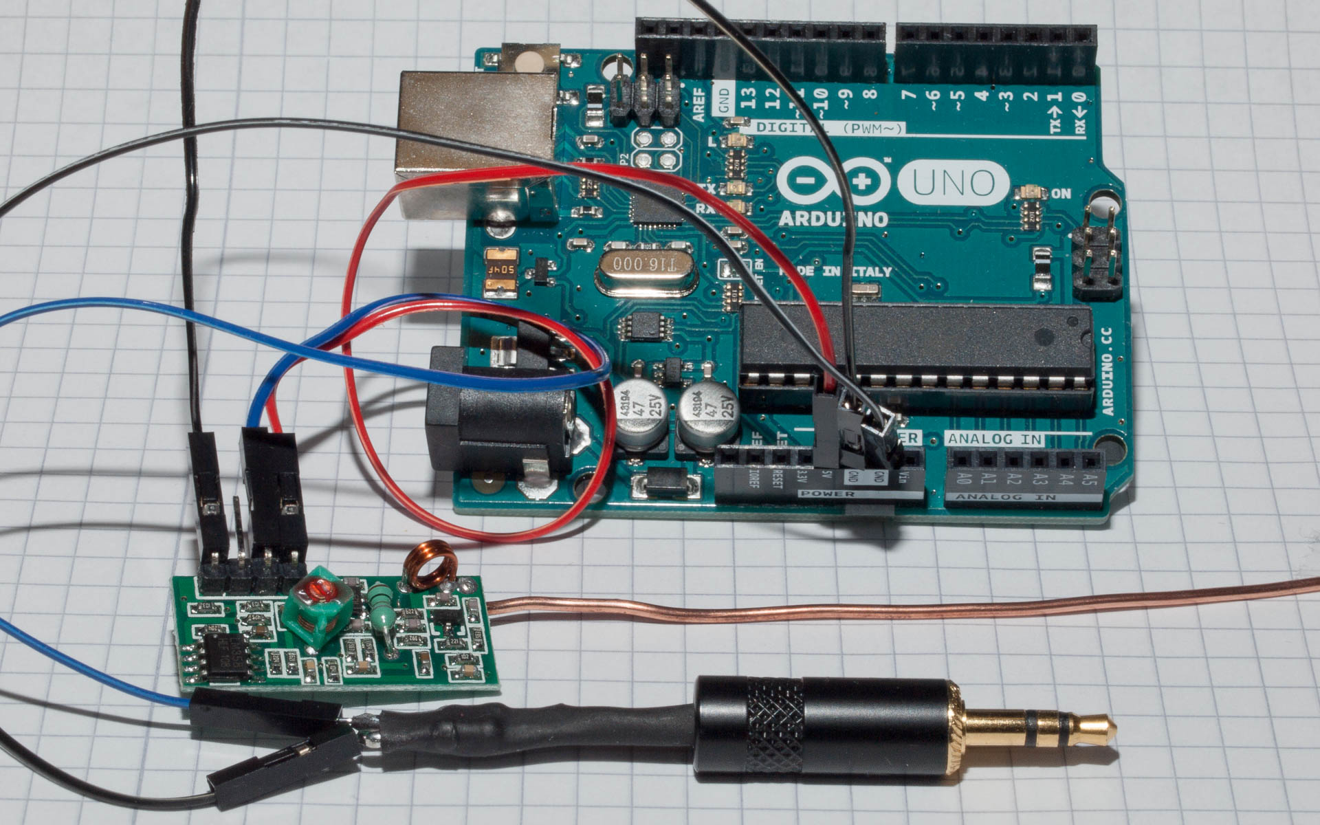
Even though microcontroller projects are usually hardware centric, the
main emphasis has been placed on the software part. My current setup utilizes
an Arduino Uno, but atMETEO is prepared to be built for different
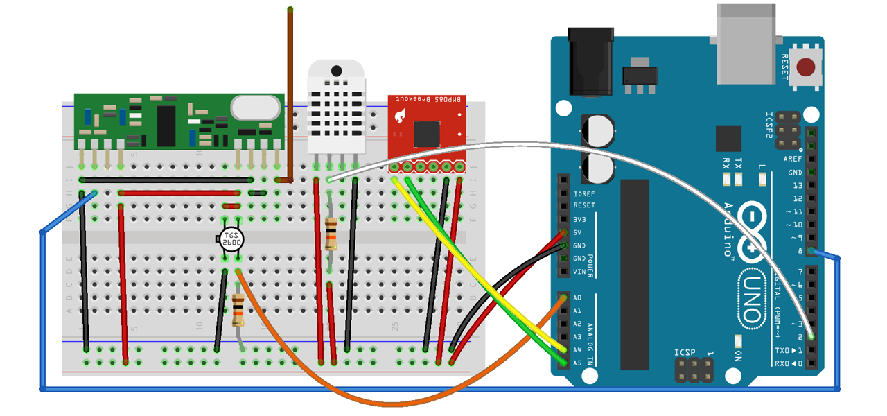
ATmega boards with only minor adaption. Currently there are 5 sensor types
supported: Hideki TS53 Thermo/Hygrometer, DHT22 / AM2302 temperature and
humidity module, Bosch BMP180 Digital pressure sensor, Melexis MLX90614
Infrared thermometer and Figaro TGS 2600 air contaminant sensor. The RF
receiver as well as the other sensors are connected to the microcontroller as
shown in the following breadboard circuit (created with Fritzing).
On the software side the project is divided into two main parts.
A libsensors library contains the target / platform independent
functionality and algorithms and ships with unit tests that can be executed
on the host. All utilities for accessing ATmega hardware features (such as
pins, timers, UART, I2C (TWI), SPI) as well as an Ethernet driver
(WIZnet W5100) are part of libtarget. The main application makes then use of
both libraries in order to send the measured sensor data in JSON format over
UART or Ethernet (UDP) to the host.
atMETEO uses the CMake build system which controls cross compilation
(including flashing) as well as unit tests (including code coverage
generation) and Doxygen documentation.
Detailed information can be found in the project’s readme and the
documentation.
Graphical user interface
Graphite and grafana are two excellent tools for logging and graphing time
series data. With the command line client atMETEO integrates nicely into
this setup as it can be configured to transfer measurements to graphite’s
carbon daemon.
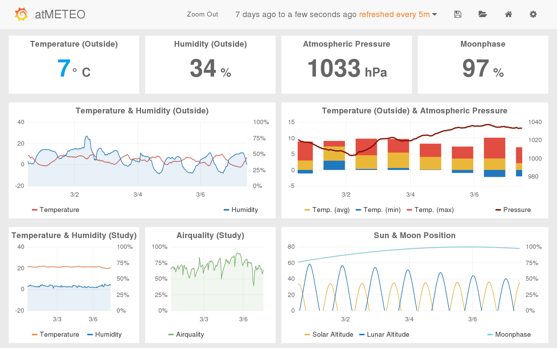
The following screenshot shows the atMETEO dashboard I am using to access
the measurements from PC, tablet or phone.
Outlook and further work
atMETEO provides weather data now since more than 10 months, even though
hardware and circuit are still just built on a breadboard. One of the very
next steps therefore is to solder the sensors on a circuit board and fit
everything into a small enclosure.
The measurements are transferred to the host in JSON format. While this is
relatively easy to generate on the microcontroller, it requires to run an
atMETEO client application on the host to interpret the data and process it.
Therefore it would be beneficial to switch to a standard format such as MQTT.
This article focuses on how to decode data sent by proprietary
RF 433 MHz sensors using the example of a wireless
thermo/hygrometer. Understanding how the sensor works is a first step towards
logging and analyzing the data on a computer.
Note that there are already implementations for many popular sensors
available online so that there’s a good chance that you will not have to
reverse engineer or implement anything on your own.
Visualizing the data
At the very beginning it is essential to understand how the basic RF signal
being transmitted looks like. This can be accomplished either with an
oscilloscope/logic analyzer or simply with a sound card, Audacity and a
voltage divider circuit limiting the 5V from the RF receiver to <1V.
When the experimental setup is functional the first step is to collect a set
of meaningful samples for the subsequent analysis. An essential part thereby
is that the original receiver is available so that the samples can be annotated
with the reference values from the receiver’s display.
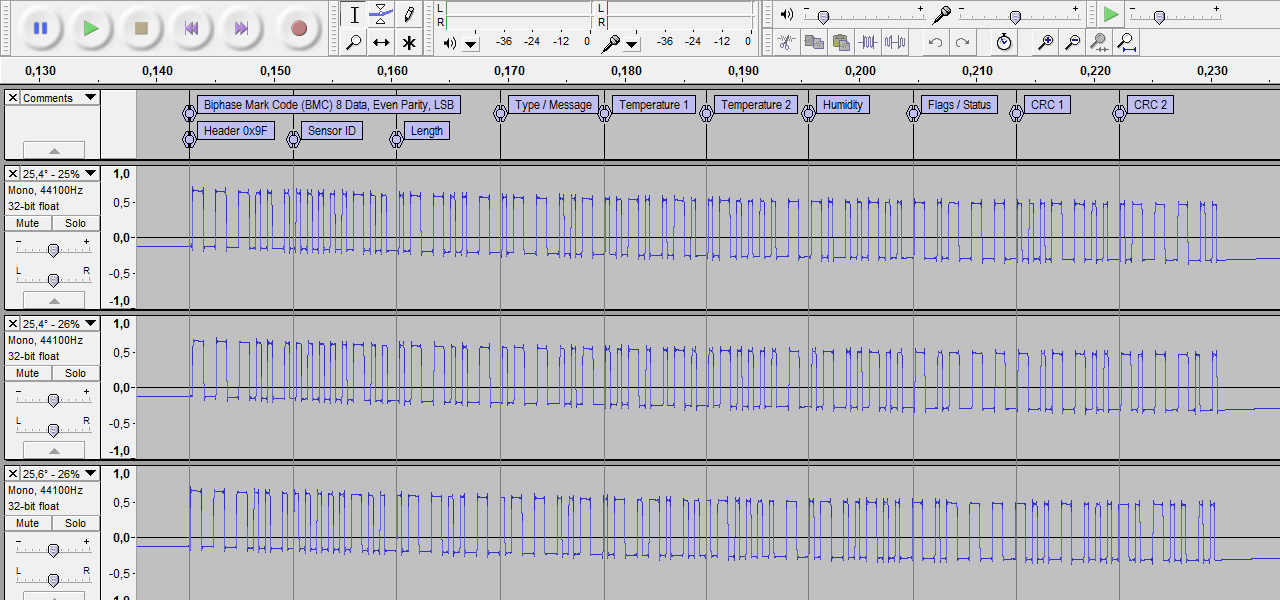
It proved to be useful to record samples that differentiate only in exactly one
value. This technique allows to easily isolate length and position of that
metric in the raw signal. Assuming that the length of a metric remains constant
for the whole message it can be used to split the message into blocks.
For the example sensor the first analysis reveals the position of temperature
and humidity as well as a block size which is illustrated by reference lines in
the figure below. It is also noticeable that the two last blocks change as soon
as temperature or humidity changes. This indicates that these blocks contain
CRC values.
The recordings should also give a good overview on how often the sender
transmits and in which time periods. The exemplary thermo/hygrometer sensor
sends three times in a row every 43 seconds.
Modulation, bit decoding and interpreting the payload
Decoding the particular sections from the example above using
Biphase Mark coding, where a long pulse represents a binary 1 and a
short pulse a binary 0, yields the following results.
The binary representation consists of ten blocks each with nine bits, which
indicates that there are eight data bits followed by one parity bit. A cross
check reveals that even parity is used.
Subsequently the binary representation has to be transformed into data bytes
by applying the correct bit numbering such as MSB or LSB. Electronic
systems commonly use Binary-coded decimal encoding a decimal digit in
four bits (nibble). Therefore bit numbering variants with reversed nibbles are
further viable options.
#1
Display
MSB 0
1
25.4° - 25%
F9 04 73 79 2A 43 A4 DF 1C 7E
2
25.4° - 26%
F9 04 73 79 2A 43 64 DF DC BD
3
25.6° - 26%
F9 04 73 79 6A 43 64 DF 9C B2
#2
Display
MSB 0 (reversed nibbles)
1
25.4° - 25%
9F 40 37 97 A2 34 4A FD C1 E7
2
25.4° - 26%
9F 40 37 97 A2 34 46 FD CD DB
3
25.6° - 26%
9F 40 37 97 A6 34 46 FD C9 2B
#3
Display
LSB 0
1
25.4° - 25%
F9 02 EC E9 45 2C 52 BF 83 E7
2
25.4° - 26%
F9 02 EC E9 45 2C 62 BF B3 DB
3
25.6° - 26%
F9 02 EC E9 65 2C 62 BF 93 D4
#4
Display
LSB 0 (reversed nibbles)
1
25.4° - 25%
9F 20 CE 9E 54 C2 25 FB 38 7E
2
25.4° - 26%
9F 20 CE 9E 54 C2 26 FB 3B BD
3
25.6° - 26%
9F 20 CE 9E 56 C2 26 FB 39 4D
For the LSB bit numbering a closer look on the values in hex shows already the
expected decimal values. The humidity can be found in byte seven (0x25 for
25%) and the temperature is located in bytes five and six. Therefore
LSB 0 with reversed nibbles seems to be the appropriate candidate for all
further proceedings.
The step of working out the correct modulation and bit numbering can be very
time consuming because the process only succeeds when at the end a correlation
between the byte value and the reference data can be found. This can make
several iterations with different parameter combinations necessary.
At the end of this process the complete user payload can be decoded which lays
the foundation for starting a basic implementation. The transmitted data
typically contains more information which can make the implementation simpler
or more robust. Examples of this are described in the next section.
Additional information encoded in the payload
Header
RF 433 MHz receivers usually perform automatic gain control to adjust
the reception level to a suitable value. While this is needed to receive data
over longer distances and to support weaker signals, it also increases the
noise level and complicates detecting the beginning of a message. Especially
because messages are only transmitted rarely in order to save energy. To
compensate this effect the messages are usually prefixed by a static pattern.
For the exemplary sensor every message starts with 0x9F.
Distinguishing sensors
If the original proprietary receiver supports multiple senders at the same
time, the protocol needs to be capable of distinguishing sensors using an ID.
The thermo/hygrometer sensor sends its ID in the second byte. The ID changes
when the battery is removed or when pushing the sensor’s reset button.
Checksums (CRCs)
CRCs are used to ensure that the data has been received correctly. Depending
on the used algorithms, they not only allow to recognize transmission errors
but also in which area of the payload it appeared and in some cases CRCs even
allow to recalculate the correct bit value. These criteria makes it interesting
trying to reverse engineer the CRCs as well.
An indication for a CRC value is a byte that changes as soon as any other bit
in the payload changes. For the exemplary sensor, this is true for the last two
bytes.
The CRC mechanisms being used can be reverse engineered using
CRC RevEng by just feeding the tool with some recorded samples.
Using the example data from the thermo/hygro sensor to decipher first CRC1 in
byte nine and then CRC2 in byte ten outputs the following CRC algorithms that
can later be implemented as explained in this article.
In addition to the fields mentioned above proprietary RF 433 MHz
protocols eventually contain more data. These are highly sensor specific so
that there is no general approach for reverse engineering those. The data
includes:
Sensor type (for generic protocols supporting different sensor types)
Payload length (if sensor sends different message types)
Sensor status
Battery information
Message id (current number of message for repeated transmission)
Conclusion
Reverse engineering proprietary RF 433 MHz sensors is possible even
with basic knowledge in electronics if the illustrated aspects are taken into
account. Especially for a first preliminary implementation not all the protocol
details are required and it is often enough to start with only the reference
data decoded. More advanced specifics like CRCs can be introduced in a later
step or left out completely if the implementation matches the quality criteria.
Recently I set up collectd, graphite and grafana to gather and visualize
statistics for the home network.
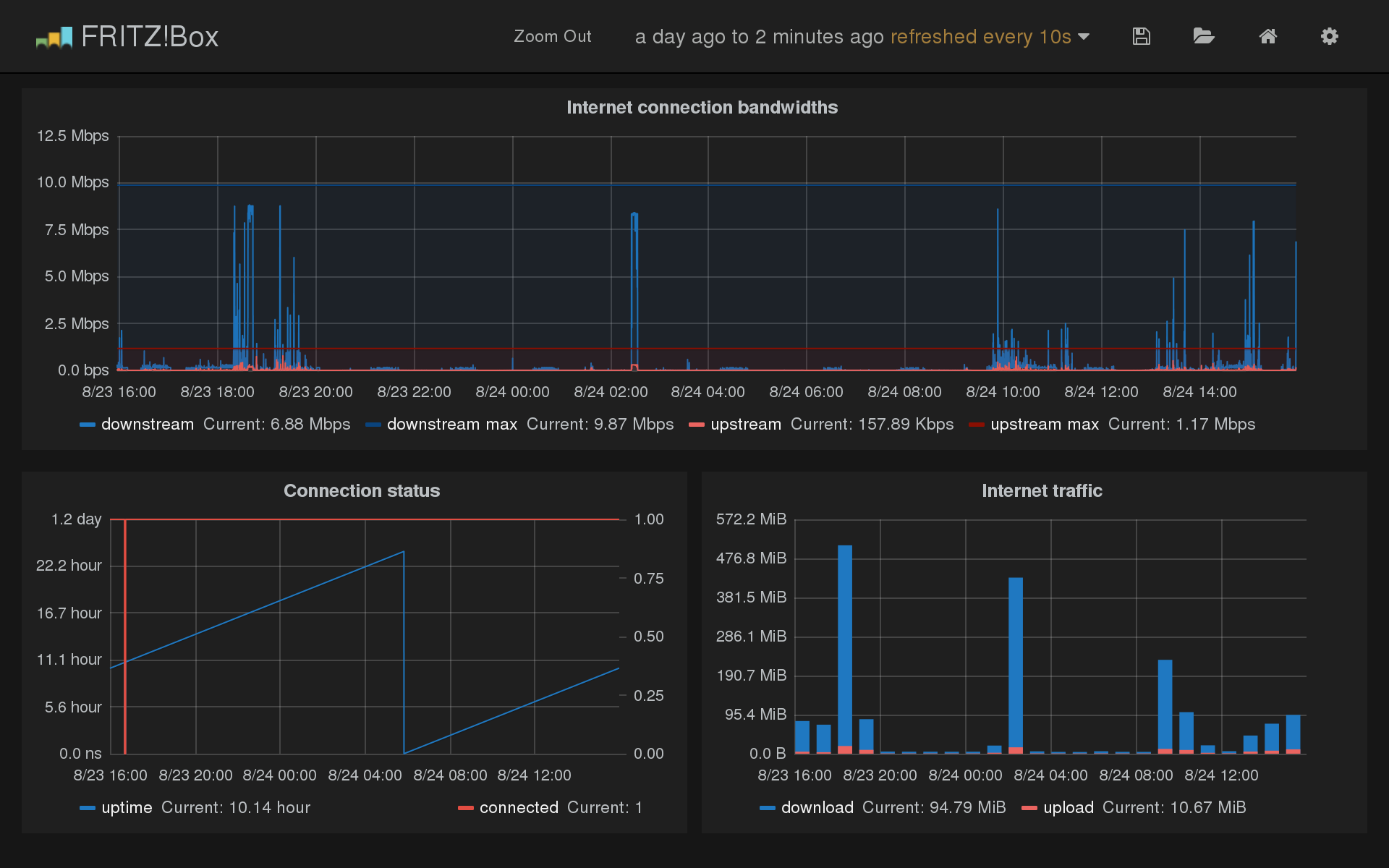
At this, I was particularly interested in monitoring my AVM FRITZ!Box router,
especially because I experience some stability problems lately.
The router exposes its status information via UPnP and fortunately there was
already a Python package available which allows to access the data from Python
scripts: fritzconnection. Hence I decided to implement a module that can feed
the data into collectd for further processing: fritzcollectd.
(see the GitHub page for installation instructions)
Since a picture is worth a thousand words, this is how it looks:
At the time of writing, there were mainly two alternative approaches documented
that are worth mentioning.
At first, there was only a snippet available which is based on a Perl script.
Besides the statistics available over UPnP the example also collects
additional data scraped from the router’s web interface.
Unfortunately even the simple version wasn’t fast enough in my environment to
retrieve the data reliably using a 10 second interval.
Secondly, if you cannot use Python or Perl plugins it is also possible to use
collectd’s cURL-XML plugin to call the respective SOAP actions directly and
parse the results with XPath.