Reverse engineering 433 MHz sensors
This article focuses on how to decode data sent by proprietary RF 433 MHz sensors using the example of a wireless thermo/hygrometer. Understanding how the sensor works is a first step towards logging and analyzing the data on a computer.
Note that there are already implementations for many popular sensors available online so that there’s a good chance that you will not have to reverse engineer or implement anything on your own.
Visualizing the data
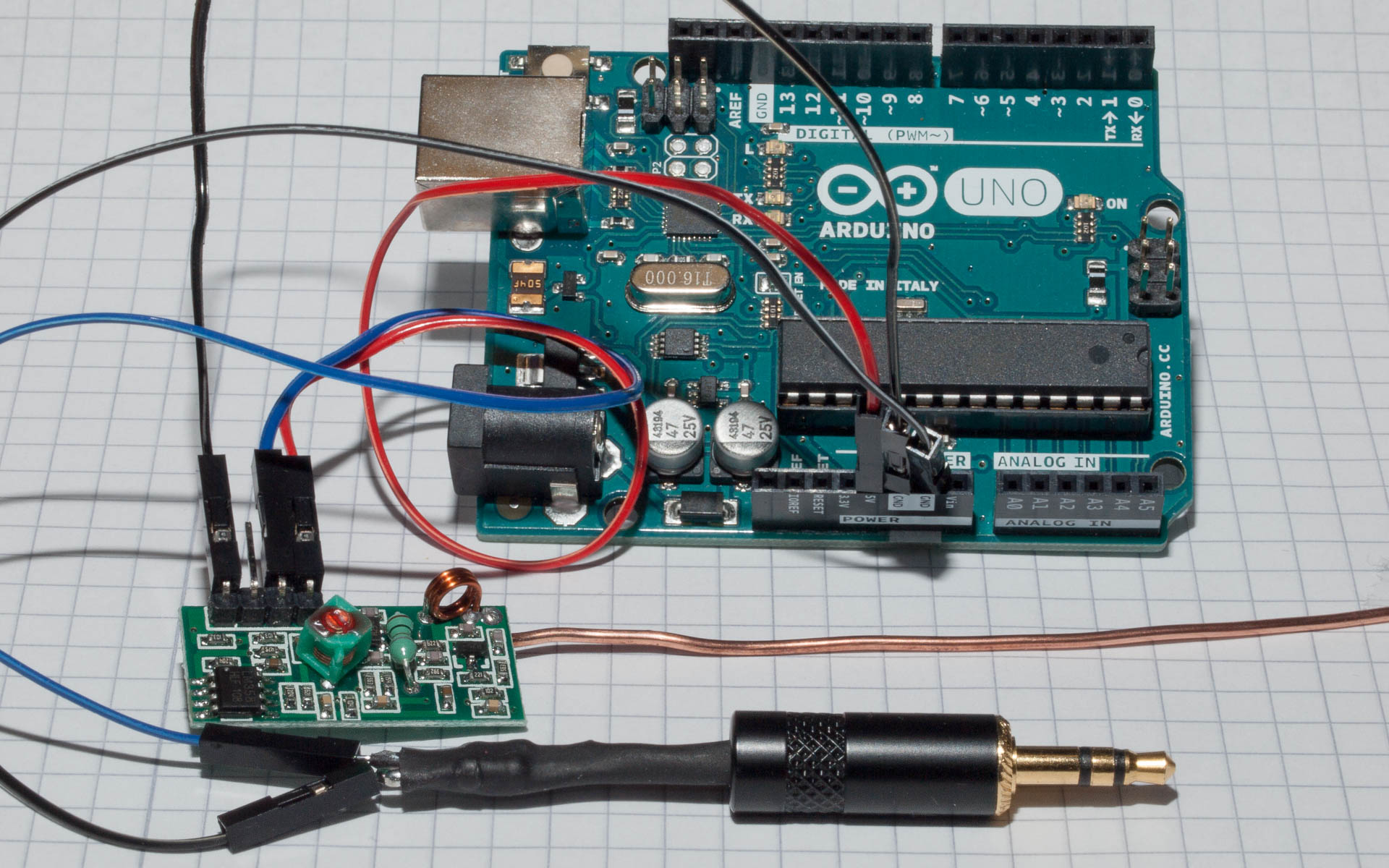
At the very beginning it is essential to understand how the basic RF signal being transmitted looks like. This can be accomplished either with an oscilloscope/logic analyzer or simply with a sound card, Audacity and a voltage divider circuit limiting the 5V from the RF receiver to <1V.
When the experimental setup is functional the first step is to collect a set of meaningful samples for the subsequent analysis. An essential part thereby is that the original receiver is available so that the samples can be annotated with the reference values from the receiver’s display. It proved to be useful to record samples that differentiate only in exactly one value. This technique allows to easily isolate length and position of that metric in the raw signal. Assuming that the length of a metric remains constant for the whole message it can be used to split the message into blocks.
For the example sensor the first analysis reveals the position of temperature and humidity as well as a block size which is illustrated by reference lines in the figure below. It is also noticeable that the two last blocks change as soon as temperature or humidity changes. This indicates that these blocks contain CRC values.
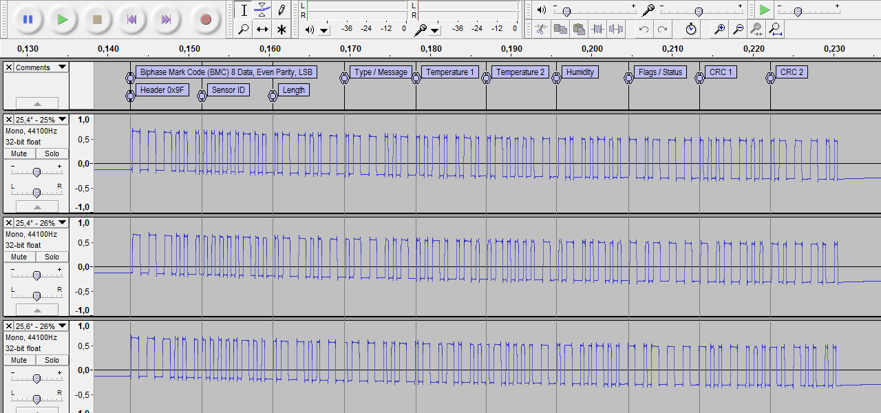
The recordings should also give a good overview on how often the sender transmits and in which time periods. The exemplary thermo/hygrometer sensor sends three times in a row every 43 seconds.
Modulation, bit decoding and interpreting the payload
The next step in the analysis is to determine which modulation is used. Typically RF 433 MHz sensors use line codes such as Manchester, Differencial Manchester or Biphase Mark coding. Other sensors use On-off keying.
Decoding the particular sections from the example above using Biphase Mark coding, where a long pulse represents a binary 1 and a short pulse a binary 0, yields the following results.
111110010 000001001 011100111 011110011 001010101 010000111 101001001 110111111 000111001 011111100
111110010 000001001 011100111 011110011 001010101 010000111 011001001 110111111 110111001 101111010
111110010 000001001 011100111 011110011 011010100 010000111 011001001 110111111 100111000 101100100
The binary representation consists of ten blocks each with nine bits, which indicates that there are eight data bits followed by one parity bit. A cross check reveals that even parity is used.
Subsequently the binary representation has to be transformed into data bytes by applying the correct bit numbering such as MSB or LSB. Electronic systems commonly use Binary-coded decimal encoding a decimal digit in four bits (nibble). Therefore bit numbering variants with reversed nibbles are further viable options.
| #1 | Display | MSB 0 |
|---|---|---|
| 1 | 25.4° - 25% | F9 04 73 79 2A 43 A4 DF 1C 7E |
| 2 | 25.4° - 26% | F9 04 73 79 2A 43 64 DF DC BD |
| 3 | 25.6° - 26% | F9 04 73 79 6A 43 64 DF 9C B2 |
| #2 | Display | MSB 0 (reversed nibbles) |
|---|---|---|
| 1 | 25.4° - 25% | 9F 40 37 97 A2 34 4A FD C1 E7 |
| 2 | 25.4° - 26% | 9F 40 37 97 A2 34 46 FD CD DB |
| 3 | 25.6° - 26% | 9F 40 37 97 A6 34 46 FD C9 2B |
| #3 | Display | LSB 0 |
|---|---|---|
| 1 | 25.4° - 25% | F9 02 EC E9 45 2C 52 BF 83 E7 |
| 2 | 25.4° - 26% | F9 02 EC E9 45 2C 62 BF B3 DB |
| 3 | 25.6° - 26% | F9 02 EC E9 65 2C 62 BF 93 D4 |
| #4 | Display | LSB 0 (reversed nibbles) |
|---|---|---|
| 1 | 25.4° - 25% | 9F 20 CE 9E 54 C2 25 FB 38 7E |
| 2 | 25.4° - 26% | 9F 20 CE 9E 54 C2 26 FB 3B BD |
| 3 | 25.6° - 26% | 9F 20 CE 9E 56 C2 26 FB 39 4D |
For the LSB bit numbering a closer look on the values in hex shows already the expected decimal values. The humidity can be found in byte seven (0x25 for 25%) and the temperature is located in bytes five and six. Therefore LSB 0 with reversed nibbles seems to be the appropriate candidate for all further proceedings.
The step of working out the correct modulation and bit numbering can be very time consuming because the process only succeeds when at the end a correlation between the byte value and the reference data can be found. This can make several iterations with different parameter combinations necessary.
At the end of this process the complete user payload can be decoded which lays the foundation for starting a basic implementation. The transmitted data typically contains more information which can make the implementation simpler or more robust. Examples of this are described in the next section.
Additional information encoded in the payload
Header
RF 433 MHz receivers usually perform automatic gain control to adjust the reception level to a suitable value. While this is needed to receive data over longer distances and to support weaker signals, it also increases the noise level and complicates detecting the beginning of a message. Especially because messages are only transmitted rarely in order to save energy. To compensate this effect the messages are usually prefixed by a static pattern. For the exemplary sensor every message starts with 0x9F.
Distinguishing sensors
If the original proprietary receiver supports multiple senders at the same time, the protocol needs to be capable of distinguishing sensors using an ID. The thermo/hygrometer sensor sends its ID in the second byte. The ID changes when the battery is removed or when pushing the sensor’s reset button.
Checksums (CRCs)
CRCs are used to ensure that the data has been received correctly. Depending on the used algorithms, they not only allow to recognize transmission errors but also in which area of the payload it appeared and in some cases CRCs even allow to recalculate the correct bit value. These criteria makes it interesting trying to reverse engineer the CRCs as well.
An indication for a CRC value is a byte that changes as soon as any other bit in the payload changes. For the exemplary sensor, this is true for the last two bytes.
The CRC mechanisms being used can be reverse engineered using CRC RevEng by just feeding the tool with some recorded samples.
Using the example data from the thermo/hygro sensor to decipher first CRC1 in byte nine and then CRC2 in byte ten outputs the following CRC algorithms that can later be implemented as explained in this article.
$ reveng -w8 -s 9F20CE9E54C225FB38 9F20CE9E54C226FB3B 9F20CE9E56C226FB39
width=8  poly=0x01  init=0x9f  refin=false  refout=false  xorout=0x00  check=0xae  name=(none)
width=8  poly=0x01  init=0xf9  refin=true  refout=true  xorout=0x00  check=0xae  name=(none)

$ reveng -w8 -s 9F20CE9E54C225FB387E 9F20CE9E54C226FB3BBD 9F20CE9E56C226FB394D
width=8  poly=0x07  init=0xf9  refin=true  refout=true  xorout=0x00  check=0x58  name=(none)
Sensor specific data
In addition to the fields mentioned above proprietary RF 433 MHz protocols eventually contain more data. These are highly sensor specific so that there is no general approach for reverse engineering those. The data includes:
- Sensor type (for generic protocols supporting different sensor types)
- Payload length (if sensor sends different message types)
- Sensor status
- Battery information
- Message id (current number of message for repeated transmission)
Conclusion
Reverse engineering proprietary RF 433 MHz sensors is possible even with basic knowledge in electronics if the illustrated aspects are taken into account. Especially for a first preliminary implementation not all the protocol details are required and it is often enough to start with only the reference data decoded. More advanced specifics like CRCs can be introduced in a later step or left out completely if the implementation matches the quality criteria.